2020. 7. 28. 22:09ㆍDeepLearning/GAN
Analyzing and Improving the Image Quality of StyleGAN

Introduction
- 제목: Analyzing and Improving the Image Quality of StyleGAN
- 저자: Tero Karras, Samuli Laine, Miika Aittala, Janne Hellsten, Jaakko Lehtinen, Timo Aila
- 기관: NVIDIA
- 요약: StyleGAN의 문제를 분석하고, 모델의 구조와 학습 방법을 개선
- Generator의 구조 개선
- Redesign generator normalization: "Droplet artifacts" 문제 해결
- Revisit progressive growing: "phase" artifacts, Shift-invariance of the network 문제 해결
- Regularze the generator : 더 좋은 image와 latent vector의 대응 (smoother latent space W)
- Capacity Increase: the effective resolution of the generated images.
- Generator에 Regularization 추가하여 더 좋은 image와 latent vector의 대응.
- Path length regularization (Perceptual Path Length의 활용)
- 생성자가 역변환(projection from images to latent space)을 하기 쉽게 한다.
- 주어진 이미지가 특정 네트워크에서 생성된 것인지 판별할 수 있다.(image forensics)
- Generator의 구조 개선
YOUTUBE : StyleGAN2
Brief review on StyleGAN

- Mapping Network : latent code z를 더욱 해석이 용이한(disentangled) 공간인 intermediate latent code w로 변환
- Style Controllability : latent code w에 아핀 변환(Affine transforms)과 AdaIN을 적용한 style은 synthesis network g 의 각 layer에서 세부적인 style의 변화 조정이 가능함
- Stochastic variation : random noise를 각 _synthesis network g_에 추가해 stochastic variation을 만든다.
- Disentanglement : The design allows intermediate latent code W to be much less entangled than the input latent space Z.
What was the problem?
StyleGAN은 기존 GAN의 생성자 구조를 바꾸어 생성된 이미지의 퀄리티에서 State-of-the-Art network였지만, 생성한 사진에 artifacts가 존재함을 확인하였다.아래 두 문제에 대하여 저자들은 이를 StyleGAN2에서 구조를 변경하면서 해결하였다.
-
Droplet artifacts: generator normalization 변경하여 해결
-
Phase artifacts: propose an alternative design that retains the benefit of progressive growing without the drawbacks
Droplet artifacts
- 최종 이미지에는 잘 안 보이더라도 feature map에서는 항상 존재
- 64 x 64 feature map을 중심으로 나타나고 점점 강해짐
- 모든 StyleGAN 이미지에 존재하였고, 만일 artifact가 생기지 않는다면 아예 잘못된 이미지가 생성
- Discriminator가 없앴어야하는 문제이지만 왜 그러지 못했는지는 저자도 의문
- solution : weight demodulation

아래 두 이미지를 비교해보면, 아주 가끔 feature map 상에서 "water droplet-like artifacts"가 생겨나지 않는 경우가 존재한다. 이러한 경우 얼굴의 특징이 normalized feature map 상에서 매우 두드러지게 나타난다. 대부분의 잘 생성된 이미지는 모두 "water droplet-like artifacts"가 있었기 때문에, StyleGAN의 생성자는 구조적 문제가 내재하고 있다고 저자들은 결론지었다.
저자들이 지적한 문제는 AdaIN이 너무 강하여 다른 정보들을 파괴하는 것이라고 한다.

We pinpoint the problem to the AdaIN operation that normalizes the mean and variance of each feature map separately, thereby potentially destroying any information found in the magnitudes of the features relative to each other. We hypothesize that the droplet artifact is a result of the generator intentionally sneaking signal strength information past instance normalization: by creating a strong, localized spike that dominates the statistics, the generator can effectively scale the signal as it likes elsewhere

- Remove (simplify) how the constant is processed at the beginning.
- The mean is not needed in normalizing the features.
- Move the noise module outside the style module.


기존 StyleGAN에서는 AdaIN이 feature map의 평균과 분산을 normalize했지만, StyleGAN2에서는 convolution weight를 normalize한다. AdaIN에서 평균을 제거하고 표준편차만 사용하였고, 표준편차만으로도 충분하다는 것을 알게 되었다. 또한. bias와 noise를 block 외부로 빼서 style과 noise의 영향력을 독립시켰다. 기존에는 noise의 영향력이 style의 크기에 반비례하였으나, noise의 변화에 따른 효과가 분명해졌다. 이는 Instance Normalization과 수학적으로 동일한 방법은 아니지만, output feature map을 standard unit standard deviation을 갖도록 해주어 학습을 더욱 안정적으로 만들며 아무튼 물방울 artifact를 없앴다.
s_i : the i th input feature map
"Even though it is not mathematically the same as the instant normalization, it normalizes the output feature map to have a standard unit standard deviation and achieve similar goals as other normalization methods (in particular, making the training more stable). Experiment results show that the blob-like artifacts are resolved."
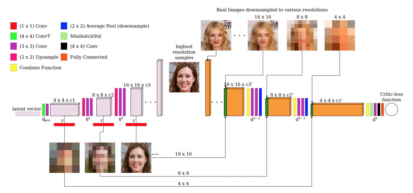
Phase artifacts
- Progressive growing appears to have strong location preference for details like teeth and eyes
- Features stay in one place before quickly moving to the next preferred location
- Authors propose an alternative design that retain the benefits of progressive growing without the drawbacks
- alternative design : training starts by focusing on low-resolution images and then progressively shifts focus to higher and higher resolution without changing the network topology during training

StyleGAN uses the progressive growth idea to stabilize the training for high-resolution images. With the progressive growth issue mentioned before, StyleGAN2 searches for alternative designs that allow network design with great depth and good training stability. For ResNet, this is done with skip connection. So StyleGAN2 explores the skip connection design and other residual concepts similar to ResNet. For these designs, we use bilinear filtering to up/downsampling the previous layers and try to learn the residual values of the next layer instead.

Style Mixing

- StyleGAN이 그러했듯, 다양한 스케일에 따라 여러 style을 섞을 수 있다.
- weight demodulation 덕분에, 생성자에서 style들은 각 scale에 잘 위치하게 된다.(즉, disentangle이 잘 된다)
- If we remove weight demodulation, the styles become cumulative rather than scale-specific
- It becomes difficult to control the image by mixing high and low-level features
- Overshooting: certain style combinations lead to artifacts
- Leaking: certain features are affected by multiple styles (e.g. background, ethnicity)
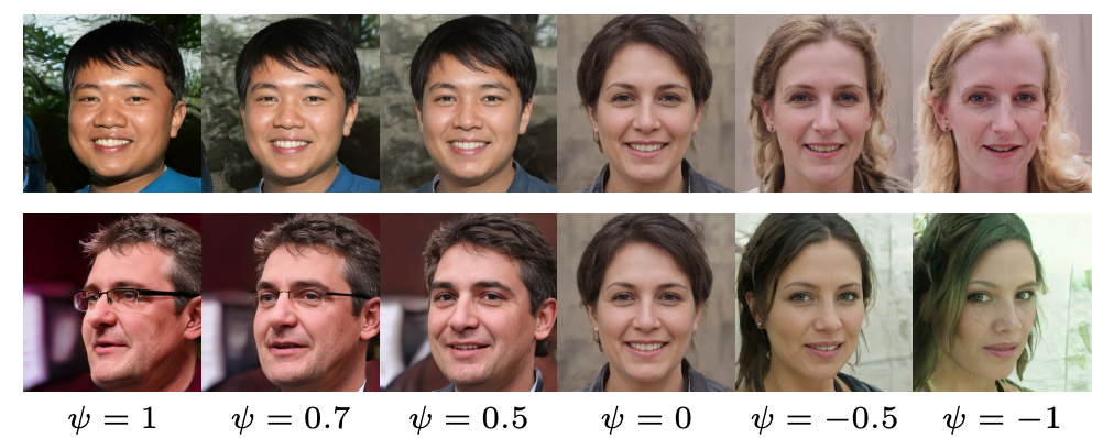
Truncation trick

if truncation < 1:
    for style in styles:
        style_t.append(
            truncation_latent + truncation * (style - truncation_latent)
        )
styles = style_t - Low truncation: high quality, limited variation
- High truncation: high variation, frequent artifacts
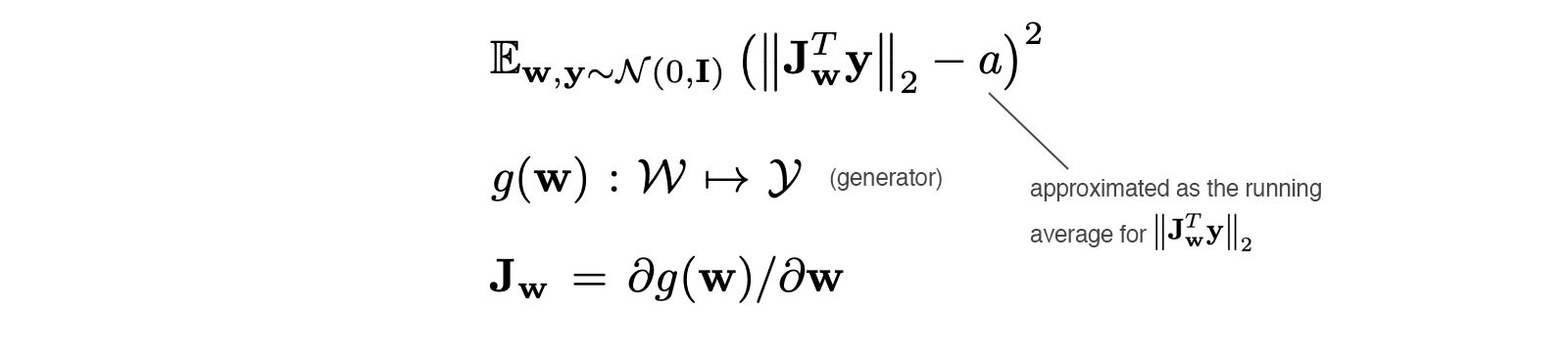
Path Length Regularization
생성 네트워크가 생성한 이미지가 실제처럼 잘 생성되었는 지를 사람이 일일이 확인 하는 것은 힘들고, 사람마다 편향이 있어 객관적이지 못하다. 이에 따라 이미지의 퀄리티를 정량적으로 평가할 기준이 필요하다. 일반적으로 generative model에 대하여 분류자(classifier) 기반의 Metric을 이용하였다.
- Fréchet Inception Distance (FID score) : measures the differences in the density of two distributions in the high dimensional feature space of a InceptionV3 classifier
- Precision and Recall (P&R): provide additional visibility by explicitly quantifying the percentage of generated images that are similar to training data and the percentage of training data can be generated, respectively.
그러나, 위 두 metric (FID and P&R)은 다음과 같은 문제가 있었다.
- 사람은 구조적(shape) 으로 잘 생성되었는 지를 기준으로 판단하지만, 네트워크는 세밀한 texture가 실제 같은 지를 기준으로 판단
저자들은 StyleGAN에서 interpolation과 disentanglement의 정량적 평가로 사용하였던 perceptual path length (PPL)이 이미지의 구조적 일관성(consistency)과 안정성(stability)과 관련되어 있다는 것을 알게 되었다.
[Smooth generator mapping]
원래 PPL은 이미지와 latent space 상에서의 대응 관계에 대한 smoothness를 측정하는 척도로 개발되었다. Latent space 상에서 노이즈를 추가하여 생성된 이미지들 상의 LPIPS distance를 측정하여 작은 값을 가질 수록 smooth하다고 하였다. 저자들은 이 현상을 잘 생성된 이미지들끼리는 좋은 latent space를 구성하였을 것이며, 잘못 생성된 이미지들(low-quality images)은 latent space상에서 작고 노이즈에 따른 변화가 큰 영역을 차지하고 있을 것이기 때문이라고 가정하였다.
We hypothesize that during training, as the discriminator penalizes broken images, the most direct way for the generator to imporve is to effectively stretch the region of latent space that yields good images.
Path Length Regularization을 적용함으로써 이미지의 퀄리티가 좋아지고, 더 나아가, 이미지로부터 latent vector를 찾아내는 역과정(inverse mapping)이 쉬워졌다고 주장한다.
Projection Method
일반적으로 이미지가 주어지면 그 이미지에 해당하는 latent code z를 optimize하는 과정이었지만, StyleGAN2에서는 (1) latent code w 와 (2) synthesis network의 각 layer에 해당하는 noise map 을 optimize하는 과정이다. 또한, Image2StyleGAN 논문에서 확장된 latent space w+을 제안하였으나 이는 학습 데이터 외에도 복원하는 (!!) 능력을 가졌기에 부적절하다고 판단하였다.
- a new method for finding the latent code that reproduces a given image
- useful for image forensics, i.e., determining whether a given image is generated or real
- 개인적으로 그냥 projection이 잘 안되는 것을 image forensic에 좋다고 한 게 아닐까...
- 생성자에 의해 생성된 이미지는 projection을 매우 잘 수행함
- 그러나 실제 이미지에 대해서는 projection이 잘 안 됨 (유사한 다른 이미지를 생성)
- StyleGAN2 generator makes it easier to distinguish generated and real images
StyleGAN2 projection method is to find the corresponding latent code w and per-layer noise maps
Optimize:
- latent code w
- per-layer noise maps
- 4x4 부터 1024x1024 까지 각 두 개씩 Noise가 들어간다. (1024x1024 의 경우 총 18개의 Noise inputs)
How to initialize?
- Initial latent code w : 10,000개의 latent code w 의 평균값
- initial noise map inputs : N(0,I)
with torch.no_grad():
     noise_sample = torch.randn(10000, 512, device = device)
     latent_out = g_ema.style(noise_sample) # mapping network f

     latent_mean = latent_out.mean(0)
     latent_std = ((latent_out - latent_mean).pow(2).sum() / n_mean_latent) ** 0.5
Adding Gaussian noise to latent code w
처음부터 3/4 구간까지 latent code w에 점진적으로 작은 gaussian noise를 더해준다. 여기에서 noise는 앞에서 설명한 synthesis network g의 각 layer에 들어가는 Noise map과는 다르다. 앞에서 임의로 뽑은 10,000개의 sample에 대하여 latent code의 standard deviation을 구한 것을 활용한다. 즉, 데이터 특성에 따른 latent space의 표준편차를 고려한 noise를 더해주어 optimization 과정에서 stochasticity를 더해주고 이상한 곳(local optimum)으로 빠지지 않도록 도와준다. 당연히 noise의 값이 너무 크면 아예 이상한 곳으로 가므로 적당한 값을 골라주어야한다. 여기에서는 0.05를 noise값으로 결정하였다.

   noise_strength = latent_std * args.noise * max(0,1 - t / args.noise_ramp) ** 2
latent_w = latent_noise(latent_w, noise_strength.item())- adds stochasticity to the optimization
- stabilizes the finding of the global optimum
Noise regularization
Given that we are explicitly optimizing the noise maps, we must be careful to avoid the optimization from sneaking actual signal into them

- Noise Regularization: sum of squares of the resolution normalized autocorrelation coefficients at one pixel shifts horizontally and vertically, which should be zero for a normally distributed signal
- Renormalization: all noise maps to N(0,1) after each optimization step.
Noise map 은 normal distribution 을 따르는데, optimization 과정에서 optimization 과정에서 signal이 noise에 들어가는 것을 방지해주어야 한다. 이에 따라 noise regularization을 주어 각 noise 사이의 correlation을 제거한다.
"We want uncorrelated Gaussian noise"
위의 regularization 항은 한 픽셀에서 인접한 픽셀 간의 normalized autocorrelation coefficient 를 의미한다.
이 값은 normal distribution 을 따를 경우 반드시 0 의 값을 가져야 한다.
또한, 각 optimization 과정마다 모든 Noise map들의 평균과 분산이 각각 0과 1이 되도록 renormalize 한다.

[References]
- https://nvlabs.github.io/stylegan2/versions.html
- https://www.youtube.com/watch?v=c-NJtV9Jvp0&feature=youtu.be
'DeepLearning > GAN' 카테고리의 다른 글
| [Paper Review] GANSpace: Discovering Interpretable GAN Controls (0) | 2020.08.27 |
|---|---|
| [Paper Review]Skip-GANomaly (0) | 2020.08.12 |
| [Paper Review] GANomaly: Semi-Supervised Anomaly Detection via Adversarial Training (0) | 2020.08.10 |
| [Paper Review] f-AnoGAN: Fast unsupervised anomaly detection with generative adversarial networks (0) | 2020.08.09 |
| [Paper Review] StyleGAN (0) | 2020.07.27 |